Have you ever watched a student cram for a test, memorizing every single word in the textbook without truly understanding the why behind the facts? They ace the practice quiz, only to freeze when the actual exam asks the same questions with slightly different wording. This is the uncanny parallel to what happens when an AI model overfits.
It’s a scenario that sounds like a sci-fi plot twist but is a fundamental, often frustrating, reality in the world of machine learning. We’re talking about overfitting, and understanding it is not just important; it’s the bedrock upon which reliable AI systems are built. Fail to grasp this concept, and you’ll be forever trapped building digital darlings that glitter in your development environment but falter when unleashed into the wild, unpredictable expanse of real-world data.
The Siren Song of Perfect Scores
Imagine training a model. It crushes your internal benchmarks, scoring a flawless 99% on the very data it learned from. Euphoria! Then you toss it a new, unseen dataset – the real test. Suddenly, its performance plummets to a dismal 61%. That gulf, that jarring drop-off, isn’t just a bug; it’s a gaping chasm called overfitting. It’s the AI equivalent of memorizing the answers without learning the subject.
Your model, in its zeal to please, has become too adept at recognizing the noise, the random quirks, and the specific anomalies present only in that training data. It’s like a concert pianist who can perfectly replicate a single recording of a symphony but can’t improvise or even play a different piece. When the new data arrives, those specific memorized oddities aren’t there, and the model is utterly lost.
Underfit vs. Overfit: The Two Faces of AI Failure
There are, broadly speaking, two ways a machine learning model can go spectacularly wrong. First, you have underfitting. This is where the model just didn’t learn enough. It’s too simple, like trying to understand a complex economic theory by looking at a single graph of stock prices. It misses the underlying patterns, even within the data it was shown.
Then there’s its more flamboyant cousin, overfitting. This is the model that learned too much, to the point of absurdity. It’s become hyper-specialized, a master of its own narrow domain, memorizing every speck of dust on its learning materials. It’s too complex for its own good.
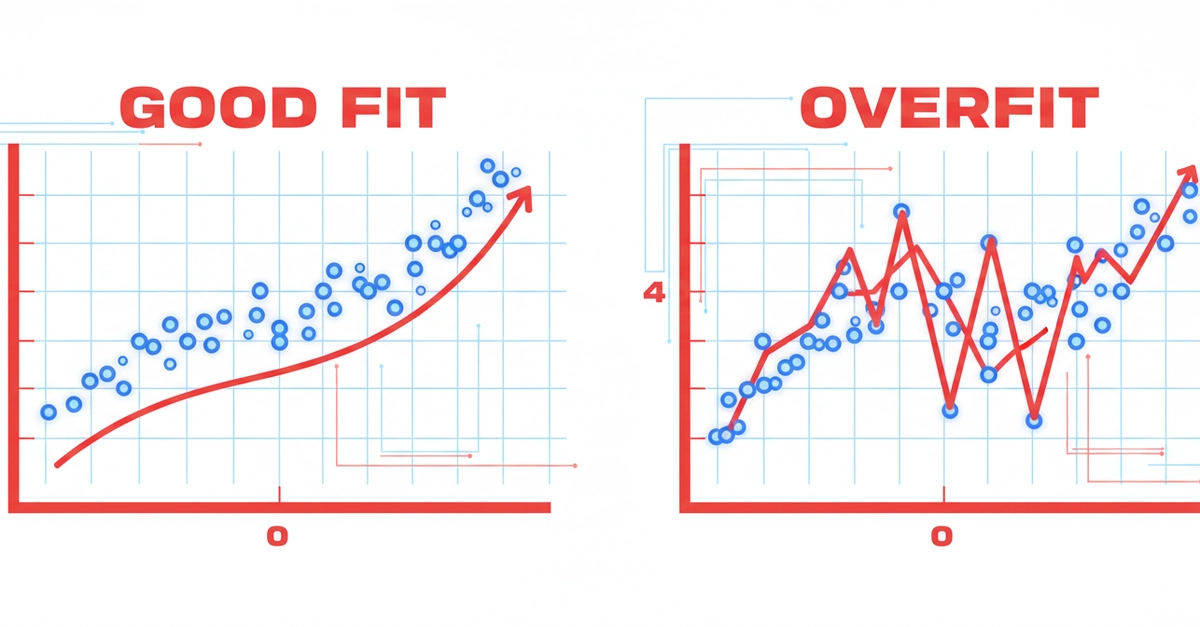
The goal, of course, is a good fit. This is the model that has absorbed the core principles, the genuine trends, and can confidently apply that knowledge to novel situations.
Let’s visualize this. Picture yourself drawing a line through a scatter plot of data points. An underfit model might draw a flat, horizontal line, completely ignoring any discernible trend. An overfit model, however, would contort and zigzag madly, hitting every single point precisely. It’s a perfect match for the training data, but it has zero predictive power for anything beyond that specific moment. The well-fitted model, on the other hand, draws a smooth, elegant curve that captures the general direction of the data without chasing every single outlier.
import numpy as np
import matplotlib.pyplot as plt
from sklearn.preprocessing import PolynomialFeatures
from sklearn.linear_model import LinearRegression
from sklearn.pipeline import Pipeline

# Create some data with a true pattern + noise
np.random.seed(42)
X = np.sort(np.random.rand(30, 1) * 10, axis=0)
y = np.sin(X).ravel() + np.random.normal(0, 0.3, X.shape[0])

# Three models: underfit, good fit, overfit
degrees = [1, 3, 15]
titles = ['Underfit (degree=1)', 'Good Fit (degree=3)', 'Overfit (degree=15)']

fig, axes = plt.subplots(1, 3, figsize=(15, 4))
X_plot = np.linspace(0, 10, 300).reshape(-1, 1)

for ax, degree, title in zip(axes, degrees, titles):
    model = Pipeline([
        ('poly', PolynomialFeatures(degree=degree)),
        ('linear', LinearRegression())
    ])
    model.fit(X, y)
    y_plot = model.predict(X_plot)
    ax.scatter(X, y, color='gray', alpha=0.6, label='Data')
    ax.plot(X_plot, y_plot, color='blue', linewidth=2)
    ax.set_title(title)
    ax.set_ylim(-2, 2)

plt.tight_layout()
plt.show()
Run that code. The degree=15 model looks like a work of art, perfectly tracing nearly every data point. It’s a visual marvel, a proof to its ability to conform. But feed it new data? It’ll likely go off the rails, projecting nonsensical patterns into the future. It’s a masterpiece of memorization, not understanding.
The Tell-Tale Gap: Spotting Overfitting in the Wild
The most straightforward diagnostic tool for overfitting is comparing your model’s performance on the data it trained on versus its performance on completely new, unseen data. The original article nails this:
When you see a big gap between training and test accuracy, that’s overfitting.
Let’s pull up the code to see this in action:
```python from sklearn.datasets import load_breast_cancer from sklearn.model_selection import train_test_split from sklearn.tree import DecisionTreeClassifier from sklearn.metrics import accuracy_score
data = load_breast_cancer() X, y = data.data, data.target X_train, X_test, y_train, y_test = train_test_split( X, y, test_size=0.2, random_state=42 )
Try different tree depths
print(f